Product Partition Models

Product-Partition Models

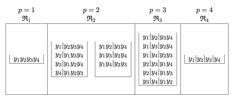
So essentially how to get \(S(n, p)\). We want to count the number of ways of partitioning \(n\) objects into \(p\) partitions. So we can write the multinomial coefficient \(\binom{n}{n_1, n_2, \dots n_p}\). This gives an ordered group i.e if \(y_1, y_2, y_3, y_4\) then \((y_1, y_2), (y_3, y_4)\) is separate from \((y_3, y_4), (y_1, y_2)\), hence we divide by \(2!\). For the more general case given in the text there are \((p-4)\) clusters of size \(a\) and \(2\) clusters of size \(b\) and \(2\) clusters of size \(c\), hence we divide by \((p-4)! 2! 2!\)

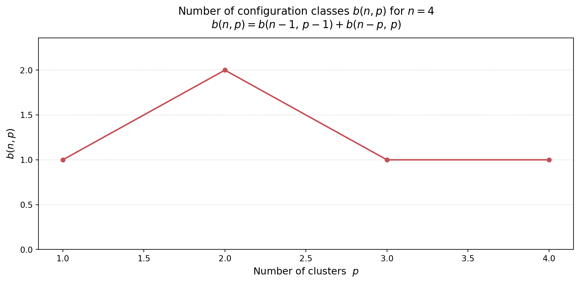
The number of configuration classes within a cluster class \(p\). Essentially how many ways can we divide up a number into \(p\) parts. If n = 4, and p = 2 then its two ways \(1, 3\) and \(2,2\). This is given by \(b(n, p)\). So if we have \(n\) items then the number of ways to form \(p\) clusters out of them is \(b(n, p)\). And \(b(n, p) = b(n-1, p-1) + b(n-p, p), 1 \leq p \leq n\) and \(b(n, 1) = 1, b(n, n) = 1\)

import numpy as np
import matplotlib.pyplot as plt
import pandas as pd 
from functools import lru_cache
import matplotlib.ticker as ticker

# ------------------------------------------------------------
# Recurrence:  b(n,p) = b(n-1,p-1) + b(n-p,p)
# Base cases:  b(n,1) = 1,  b(n,n) = 1
# ------------------------------------------------------------
@lru_cache(maxsize=None)
def b(n, p):
    if p < 1 or p > n:
        return 0
    if p == 1 or p == n:
        return 1
    return b(n - 1, p - 1) + b(n - p, p)


n      = 4
p_vals = list(range(1, n + 1))
b_vals = [b(n, p) for p in p_vals]

# ------------------------------------------------------------
# Plot
# ------------------------------------------------------------
fig, ax = plt.subplots(figsize=(10, 5))

# Overlay line + markers
ax.plot(p_vals, b_vals, color="#C44E52", linewidth=1.8,marker="o", markersize=5, zorder=4)
ax.set_xlabel("Number of clusters  $p$", fontsize=12)
ax.set_ylabel("$b(n,p)$", fontsize=12)
ax.set_title(
    "Number of configuration classes $b(n,p)$ for $n = 4$\n"
    r"$b(n,p) = b(n-1,\,p-1) + b(n-p,\,p)$",
    fontsize=13, pad=12
)

ax.grid(axis="y", linestyle="--", linewidth=0.6, alpha=0.5, zorder=0);
ax.set_ylim(0, max(b_vals) * 1.18);

plt.tight_layout();
plt.show()

So there are greater number of ways to divide a group of 4 objects into 2 clusters than to divide them into 1 or 3 or 4 clusters. Within each clusters class e.g. for 2 clusters class there are 7 clusters possible , for 4 and 1 clusters there is only 1 and for 3 there are 6 clusters possible. Now \(R_p = \sum_{n_c } R_{n_c, p}\) where I have \(R_2 = R_{(4 = 1+3), 2} + R_{(4 = 2+ 2), 2}\) and of course this number is much greater than \(b(n, p) = 2\). For this case \(R_2 = 7\)

Known issues with Mixture Models. 1. In mixture models, label switching comes from the fact that component labels (1, 2, …, K) are arbitrary — swapping them does not change the model or likelihood. This is because we usually do \(\sum_k \pi_k L(x|k)\) and hence we can switch the labeling on the parameters. In MCMC, this causes the chain to move between equivalent parameterizations (e.g., component 1 and 2 swapping roles), because it explores the full symmetric posterior. In EM or gradient descent, there is no switching during optimization; instead, the algorithm converges to one of the equivalent optima depending on initialization. Different runs may end up with permuted labels.

So we introduce product partition models the notation is a bit clunky but its pretty self-explanatory. We need a prior over \(p, r_p, \theta_p\) where \(p\) is number of clusters we want \(r_p\) is the partition ie partition of each point \(n_i\) into one of \(p\) clusters. Basically use Bayes rule etc. etc. to define the relevant quatitities above. Additionally define the Bayes factor \(\frac{m(y| r_p, n)}{m(y | r_1, n)}\) which defines how well a particular partition is supported over the partition of size \(1\).

Selecting priors for the clustering model…

Uniform Prior over Partitions.
Ewens - Pitman Prior
Jensen-Liu Prior
HUP (This paper…) - Basically defined by assuming that things are uniform within data generating process proposed above…

Ok so i could look into what Ewens-Pitman and Jensen-Liu are I dont know how these priors are derived… But Table 1. shows the uniform prior assigns more weight to the entropically favorable partition while for Ewens-Pitman and Jensen-Liu the situations are reversed i.e they favor \({1, 3, 6}\) over \({2, 3, 5}\) for \(R_{10, 3}\) where the prior numbers are sizes of the clusters and \(\lambda = 1\) for both Ewens-Pitman and Jensen-Liu.

The HUP however - says that \(p\) should be small since we want a smaller number of clusters this is debatable… Alright but the way we derive the prior is

Say that \(P(p | \lambda)\) is a Poisson and \(P(\lambda)\) is Jeffery’s Prior and now integrate out \(\lambda\) to get \(P(p| n)\) where we truncate the to the set \(1...n\) since \(p\) cannot be greater than \(n\). We can get different tail behaviors by choosing different kinds of priors for the \(\lambda\) parameter.

So the HUP says

Select \(p\) ie number of clusters we want
Select one of \(b(n, p)\) uniformly ie. which one of the \(p\) ways of partitioning \(n\) we want i.e. whether \(4 = 1 + 3\) or \(4 = 2 + 2\)
Assign uniform probabilities to all partitions within \(R_p\) i.e within all cluster of class \(1, 3\) all partitions are uniform and so on…

Jensen-Liu and Uniform favor large number of clusters with fewer points in each cluster. While Ewens-Pitman and HUP are better with HUP having a faster convergence rate.

References

Cluster Analysis, Model Selection, and Prior Distributions on Models, George Casella, Elías Moreno, F. Javier Girón