Gaussian Belief Propagation on Trees
Introduction
Efficient inference on models represented by large, dynamic, and highly inter-connected graphs is challenging.
Belief Propagation (BP)
Belief Propagation is an algorithm used for calculating the marginals of a joint distribution via local message passing between nodes in a factor graph.
Factor Graphs
Factor graphs are a type of bipartite graphical model that connects variables via factors. These factors represent the local dependencies between the variables.
Performance and Convergence
- Tree-structured graphs: BP is exact.
- Loopy graphs: BP is an approximation but empirically produces high-quality results.
Gaussian Belief Propagation (GBP)
GBP specifically addresses cases where the distributions are Gaussian. Key characteristics include: - Linear Systems: GBP is closely linked to solving linear systems. (Why ???, Schur’s complement) - Extensions: Handling non-linearities and non-Gaussian data. (Just the laplace approximation)
Mathematical Foundation
According to the Hammersley-Clifford Theorem, the joint probability distribution factorizes as: \[ p(X) = \prod_{i} f_i(X_i) \]
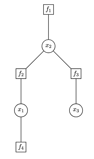
Example Factor Graph
For a system with variables \(x_1, x_2, x_3\), the joint distribution is: \[ p(x_1, x_2, x_3) = f_1(x_1) f_2(x_2) f_3(x_1, x_2) f_4(x_2, x_3) \]
BP Equations
Factors are basically all the independent factors that appear in the joint distribution.
Factor to Variable Message: Product of all messages from all variable nodes except \(i\) to the factor node \(f_j\) times the factor and then integrate out all the \(x_j\) except \(x_i\) \[ m_{f_j \to x_i} = \sum_{x_{j \setminus i}} \left( \prod_{k \in N(j) \setminus i} m_{x_k \to f_j} \right) (f_j(x_j)) \]
Variable to Factor Message: Product of all messages incoming to the variable except from the factor the message is being sent to \[ m_{x_i \to f_j} = \prod_{s \in N(i) \setminus j} m_{f_s \to x_i} \]
Belief Update: Product of all messages incoming to a variable \[ b_i(x_i) = \prod_{s \in N(i)} m_{f_s \to x_i} \]
Gaussian Forms
Moments Form: \[ E(x) = \frac{1}{2}(x-\mu)^T \Sigma^{-1} (x-\mu) \]
Canonical Form: \[ E(x) = \frac{1}{2}x^T \Lambda x - \eta^T x \] Where \(\Lambda = \Sigma^{-1}\) (Precision) and \(\eta = \Sigma^{-1}\mu\) (Information vector).
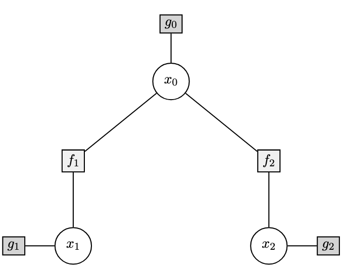
Doing the derivation for a small example tree.
Message Passing Equations
1. Leaf to Variable Messages
The messages from the evidence factors \(g_1\) and \(g_2\) to the variable nodes are given by Gaussians: \[ m_{g_2 \to x_2} = \mathcal{N}(x_2 | \mu_2, \sigma_2^2) \] \[ m_{g_1 \to x_1} = \mathcal{N}(x_1 | \mu_1, \sigma_1^2) \]
2. Variable to Factor Messages
Since \(x_1\) and \(x_2\) only have one incoming message from the leaves: \[ m_{x_1 \to f_1} = m_{g_1 \to x_1} \] \[ m_{x_2 \to f_2} = m_{g_2 \to x_2} \]
3. Factor to Variable Messages (Marginalization)
The messages from factors \(f_1\) and \(f_2\) to the root node \(x_0\) are computed by integrating out the leaf variables: \[ m_{f_2 \to x_0} = \int f_2 \cdot m_{x_2 \to f_2} \, dx_2 \] \[ m_{f_1 \to x_0} = \int f_1 \cdot m_{x_1 \to f_1} \, dx_1 \]
Evaluation of the Integrals
Taking the message \(m_{f_2 \to x_0}\) as an example: \[ m_{f_2 \to x_0} = \int \frac{1}{\sqrt{2\pi t_2 v}} e^{-\frac{1}{2}\frac{(x_0 - x_2)^2}{t_2 v}} \frac{1}{\sqrt{2\pi \sigma_2^2}} e^{-\frac{1}{2}\frac{(x_2 - \mu_2)^2}{\sigma_2^2}} \, dx_2 \]
Solving the Gaussian convolution (completing the square), we get:
\[ \int \frac{1}{\sqrt{2\pi t_2 v}} e^{-\frac{1}{2} \frac{(x_0 - x_2)^2}{t_2 v}} \frac{1}{\sqrt{2\pi \sigma_2^2}} e^{-\frac{1}{2} \frac{(x_2 - \mu_2)^2}{\sigma_2^2}} dx_2 \] \[ = \frac{1}{2\pi} \times \frac{1}{\sqrt{t_2 v}} \times \frac{1}{\sqrt{\sigma_2^2}} \exp \left[ -\frac{1}{2} \left[ \frac{x_0^2}{t_2 v} + \frac{x_2^2}{t_2 v} - \frac{2x_0 x_2}{t_2 v} + \frac{x_2^2}{\sigma_2^2} + \frac{\mu_2^2}{\sigma_2^2} - \frac{2x_2 \mu_2}{\sigma_2^2} \right] \right] \] \[ = \frac{1}{2\pi \sqrt{t_2 v \sigma_2^2}} e^{-\frac{1}{2} \left[ x_2^2 \left( \frac{1}{t_2 v} + \frac{1}{\sigma_2^2} \right) - 2x_2 \left[ \frac{x_0}{t_2 v} + \frac{\mu_2}{\sigma_2^2} \right] + \frac{x_0^2}{t_2 v} + \frac{\mu_2^2}{\sigma_2^2} \right]} \] \[ = \frac{1}{2\pi \sqrt{t_2 v \sigma_2^2}} e^{-\frac{1}{2} \left( \frac{1}{t_2 v} + \frac{1}{\sigma_2^2} \right) \left[ x_2^2 - 2x_2 \left( \frac{\frac{x_0}{t_2 v} + \frac{\mu_2}{\sigma_2^2}}{\frac{1}{t_2 v} + \frac{1}{\sigma_2^2}} \right) + \frac{\frac{x_0^2}{t_2 v} + \frac{\mu_2^2}{\sigma_2^2}}{\frac{1}{t_2 v} + \frac{1}{\sigma_2^2}} \right]} \] \[ = \frac{1}{2\pi \sqrt{t_2 v \sigma_2^2}} e^{-\frac{1}{2} \left( \frac{1}{t_2 v} + \frac{1}{\sigma_2^2} \right) \left[ \left( x_2 - \frac{\left( \frac{x_0}{t_2 v} + \frac{\mu_2}{\sigma_2^2} \right)}{\frac{1}{t_2 v} + \frac{1}{\sigma_2^2}} \right)^2 + \frac{\frac{x_0^2}{t_2 v} + \frac{\mu_2^2}{\sigma_2^2}}{\frac{1}{t_2 v} + \frac{1}{\sigma_2^2}} - \left( \frac{\frac{x_0}{t_2 v} + \frac{\mu_2}{\sigma_2^2}}{\frac{1}{t_2 v} + \frac{1}{\sigma_2^2}} \right)^2 \right]} \] \[ = \frac{1}{2\pi \sqrt{t_2 v \sigma_2^2}} e^{-\frac{1}{2} \left( \frac{1}{t_2 v} + \frac{1}{\sigma_2^2} \right) \left( x_2 - \frac{\left( \frac{x_0}{t_2 v} + \frac{\mu_2}{\sigma_2^2} \right)}{\frac{1}{t_2 v} + \frac{1}{\sigma_2^2}} \right)^2} e^{-\frac{1}{2} \left[ \left( \frac{x_0^2}{t_2 v} + \frac{\mu_2^2}{\sigma_2^2} \right) - \frac{\left( \frac{x_0}{t_2 v} + \frac{\mu_2}{\sigma_2^2} \right)^2}{\frac{1}{t_2 v} + \frac{1}{\sigma_2^2}} \right]} \] \[ = \frac{1}{2\pi \sqrt{t_2 v \sigma_2^2}} \times \sqrt{\frac{2\pi}{\frac{1}{t_2 v} + \frac{1}{\sigma_2^2}}} \times e^{-\frac{1}{2} \left[ \frac{x_0^2}{t_2 v^2} + \frac{\mu_2^2}{\sigma_2^4} + \frac{x_0^2}{t_2 \sigma_2^2} + \frac{\mu_2^2}{\sigma_2^2 t_2 v} - \frac{x_0^2}{t_2 v^2} - \frac{\mu_2^2}{\sigma_2^4} - \frac{2x_0 \mu_2}{t_2 v \sigma_2^2} \right] / \left( \frac{1}{t_2 v} + \frac{1}{\sigma_2^2} \right)} \] \[ = \frac{1}{\sqrt{2\pi (t_2 v + \sigma_2^2)}} e^{-\frac{1}{2} \frac{(x_0 - \mu_2)^2}{(\frac{1}{t_2 v} + \frac{1}{\sigma_2^2})(t_2 v \sigma_2^2 )}} \] \[ = \frac{1}{\sqrt{2\pi (t_2 v + \sigma_2^2)}} e^{-\frac{1}{2} \frac{(x_0 - \mu_2)^2}{t_2 v + \sigma_2^2}} \]
\[ m_{f_2 \to x_0} = \frac{1}{\sqrt{2\pi (\sigma_2^2 + t_2 v)}} e^{-\frac{1}{2} \frac{(x_0 - \mu_2)^2}{t_2 v + \sigma_2^2}} \]
Similarly for \(m_{f_1 \to x_0}\): \[ m_{f_1 \to x_0} = \frac{1}{\sqrt{2\pi (\sigma_1^2 + t_1 v)}} e^{-\frac{1}{2} \frac{(x_0 - \mu_1)^2}{t_1 v + \sigma_1^2}} \]
Partition Function and Total Probability
The partition function \(Z\) (which equals the probability of the data \(P(D)\)) is the integral over \(x_0\), assuming \(m_{g_0 \to x_0}\) is uniform. \[ Z = P(D) = \int m_{f_2 \to x_0} \cdot m_{f_1 \to x_0} \cdot m_{g_0 \to x_0} \, dx_0 \]
\[ Z = \int \frac{1}{2\pi \sqrt{V_1 V_2}} e^{-\frac{1}{2} \left[ \frac{(x_0 - \mu_1)^2}{V_1} + \frac{(x_0 - \mu_2)^2}{V_2} \right]} dx_0 \] \[ = \frac{1}{\sqrt{2\pi (V_1 + V_2)}} e^{-\frac{1}{2} \frac{(\mu_1 - \mu_2)^2}{V_1 + V_2}} \]
Where: \[ V_1 = t_1 v + \sigma_1^2 \quad \text{and} \quad V_2 = t_2 v + \sigma_2^2 \]
Starting from the exponent: \[ \text{Exponent} = -\frac{1}{2} \left[ \frac{(x_0 - \mu_1)^2}{V_1} + \frac{(x_0 - \mu_2)^2}{V_2} \right] \] \[ = -\frac{1}{2} \left\{ x_0^2 \left[ \frac{1}{V_1} + \frac{1}{V_2} \right] - 2x_0 \left[ \frac{\mu_1}{V_1} + \frac{\mu_2}{V_2} \right] + \frac{\mu_1^2}{V_1} + \frac{\mu_2^2}{V_2} \right\} \] \[ = -\frac{1}{2} \left( \frac{1}{V_1} + \frac{1}{V_2} \right) \left[ x_0^2 - 2x_0 \left( \frac{\frac{\mu_1}{V_1} + \frac{\mu_2}{V_2}}{\frac{1}{V_1} + \frac{1}{V_2}} \right) + \frac{\frac{\mu_1^2}{V_1} + \frac{\mu_2^2}{V_2}}{\frac{1}{V_1} + \frac{1}{V_2}} \right] \] \[ = -\frac{1}{2} \left( \frac{1}{V_1} + \frac{1}{V_2} \right) \left[ \left( x_0 - \frac{\frac{\mu_1}{V_1} + \frac{\mu_2}{V_2}}{\frac{1}{V_1} + \frac{1}{V_2}} \right)^2 + \frac{\frac{\mu_1^2}{V_1} + \frac{\mu_2^2}{V_2}}{\frac{1}{V_1} + \frac{1}{V_2}} - \left( \frac{\frac{\mu_1}{V_1} + \frac{\mu_2}{V_2}}{\frac{1}{V_1} + \frac{1}{V_2}} \right)^2 \right] \] \[ = -\frac{1}{2} \left( \frac{1}{V_1} + \frac{1}{V_2} \right) \left( x_0 - \frac{\frac{\mu_1}{V_1} + \frac{\mu_2}{V_2}}{\frac{1}{V_1} + \frac{1}{V_2}} \right)^2 - \frac{1}{2} \left( \frac{1}{V_1} + \frac{1}{V_2} \right) \left[ \frac{\frac{\mu_1^2}{V_1} + \frac{\mu_2^2}{V_2}}{\frac{1}{V_1} + \frac{1}{V_2}} - \left( \frac{\frac{\mu_1}{V_1} + \frac{\mu_2}{V_2}}{\frac{1}{V_1} + \frac{1}{V_2}} \right)^2 \right] \]
Integrating over \(x_0\): \[ \text{Result} = \frac{\sqrt{2\pi}}{\sqrt{\frac{1}{V_1} + \frac{1}{V_2}}} e^{-\frac{1}{2} \left[ \frac{\left( \frac{\mu_1^2}{V_1} + \frac{\mu_2^2}{V_2} \right) \left( \frac{1}{V_1} + \frac{1}{V_2} \right) - \left( \frac{\mu_1}{V_1} + \frac{\mu_2}{V_2} \right)^2}{\frac{1}{V_1} + \frac{1}{V_2}} \right]} \] \[ = \frac{1}{2\pi \sqrt{V_1 V_2}} \times \sqrt{\frac{2\pi V_1 V_2}{V_1 + V_2}} e^{-\frac{1}{2} \left[ \frac{\mu_1^2 + \mu_2^2 - 2\mu_1 \mu_2}{V_1 + V_2} \right]} \] \[ = \frac{1}{\sqrt{2\pi (V_1 + V_2)}} e^{-\frac{1}{2} \frac{(\mu_1 - \mu_2)^2}{V_1 + V_2}} \]
Beliefs (Marginals)
The beliefs are the marginals computed by taking the product of all incoming messages to that node: \[ b(x_2) \propto m_{f_2 \to x_2} \cdot m_{g_2 \to x_2} \] \[ b(x_1) \propto m_{f_1 \to x_1} \cdot m_{g_1 \to x_1} \] \[ b(x_0) \propto m_{f_2 \to x_0} \cdot m_{f_1 \to x_0} \cdot m_{g_0 \to x_0} \]
Precision Matrix and Schur Complement
Precision Matrix Formulation and Gaussian Elimination
\[ Q = \begin{array}{c|ccccc} & x_0 & x_1 & x_2 & \mu_2 & \mu_1 \\ \hline x_0 & \frac{1}{t_2 v} + \frac{1}{t_1 v} & -\frac{1}{t_1 v} & -\frac{1}{t_2 v} & 0 & 0 \\ x_1 & -\frac{1}{t_1 v} & \frac{1}{t_1 v} + \frac{1}{\sigma_1^2} & 0 & 0 & -\frac{1}{\sigma_1^2} \\ x_2 & -\frac{1}{t_2 v} & 0 & \frac{1}{t_2 v} + \frac{1}{\sigma_2^2} & -\frac{1}{\sigma_2^2} & 0 \\ \mu_2 & 0 & 0 & -\frac{1}{\sigma_2^2} & \frac{1}{\sigma_2^2} & 0 \\ \mu_1 & 0 & -\frac{1}{\sigma_1^2} & 0 & 0 & \frac{1}{\sigma_1^2} \end{array} \]
The joint distribution is factored as: \[ p(x_2, \mu_2, x_1, x_0, \mu_1) = p(x_2 | x_0) p(\mu_2 | x_2) p(x_1 | x_0) p(\mu_1 | x_1) p(x_0) \] which can be written in terms of the precision matrix \(Q\): \[ p(x, y) \propto \exp \left( -\frac{1}{2} \sum_{i,j} Q_{ij} x_i x_j \right) \]
By matching terms in the joint distribution, we identify the entries of \(Q\) (e.g., \(Q_{x_0, x_0} = \frac{1}{t_2 v} + \frac{1}{t_1 v}\) and \(Q_{x_1, x_0} = -\frac{1}{t_1 v}\)).
We partition the state vector into \(\mathbf{x}\) (internal nodes) and \(\mathbf{y}\) (leaf/parameter nodes): \[ \mathbf{x} = \begin{pmatrix} x_0 \\ x_1 \\ x_2 \end{pmatrix}, \quad \mathbf{y} = \begin{pmatrix} \mu_2 \\ \mu_1 \end{pmatrix} \quad \Rightarrow \quad Q = \begin{bmatrix} A & B \\ B^T & C \end{bmatrix} \]
The log-probability is given by: \[ \log P(\{\mathbf{x}, \mathbf{y}\}) \propto -\frac{1}{2} \begin{pmatrix} \mathbf{x} \\ \mathbf{y} \end{pmatrix}^T \begin{bmatrix} A & B \\ B^T & C \end{bmatrix} \begin{pmatrix} \mathbf{x} \\ \mathbf{y} \end{pmatrix} \]
To integrate out \(\mathbf{x}\) (marginalization), we complete the square, resulting in the marginal precision matrix for \(\mathbf{y}\): \[ Q_y = C - B^T A^{-1} B \]
Where the sub-matrices are defined as: \[ A = \begin{bmatrix} \frac{1}{t_2 v} + \frac{1}{t_1 v} & -\frac{1}{t_1 v} & -\frac{1}{t_2 v} \\ -\frac{1}{t_1 v} & \frac{1}{t_1 v} + \frac{1}{\sigma_1^2} & 0 \\ -\frac{1}{t_2 v} & 0 & \frac{1}{t_2 v} + \frac{1}{\sigma_2^2} \end{bmatrix}, \quad B = \begin{bmatrix} 0 & 0 \\ 0 & -\frac{1}{\sigma_1^2} \\ -\frac{1}{\sigma_2^2} & 0 \end{bmatrix}, \quad C = \begin{bmatrix} \frac{1}{\sigma_2^2} & 0 \\ 0 & \frac{1}{\sigma_1^2} \end{bmatrix} \]
Another way to do the derivation
We can also write: \[ \mu_1 = x_1 + \sigma_1 \zeta_1 \] \[ x_1 = x_0 + \sqrt{t_1 v} \zeta_2 \]
where \(\zeta_1, \zeta_2 \sim \mathcal{N}(0, 1)\) are independent standard normal random variables. Substituting \(x_1\) into the equation for \(\mu_1\), we get: \[ \mu_1 = x_0 + \sqrt{t_1 v} \zeta_2 + \sigma_1 \zeta_1 \]
By the property of the convolution of Gaussians, the sum of two independent zero-mean Gaussians \(\mathcal{N}(0, \sigma_1^2)\) and \(\mathcal{N}(0, t_1 v)\) is itself a Gaussian \(\mathcal{N}(0, \sigma_1^2 + t_1 v)\). Thus, we can simplify the expression to: \[ \mu_1 = x_0 + \sqrt{\sigma_1^2 + t_1 v} \zeta_1 \] where \(\zeta \sim \mathcal{N}(0, 1)\). Similarly, for the second branch of the tree: \[ \mu_2 = x_0 + \sqrt{\sigma_2^2 + t_2 v} \zeta_2 \]
This allows us to write the conditional probability (likelihood) \(P(D | x_0)\) as the product of two independent Gaussian distributions: \[ P(D | x_0) = \frac{1}{2\pi \sqrt{V_1 V_2}} \exp \left( -\frac{1}{2} \left[ \frac{(x_0 - \mu_1)^2}{V_1} + \frac{(x_0 - \mu_2)^2}{V_2} \right] \right) \]
Where the total variances are defined as: \[ V_1 = t_1 v + \sigma_1^2 \] \[ V_2 = t_2 v + \sigma_2^2 \]
We take a uniform prior for \(x_0\) and we have already seen how to solve this integral.
Can use this approach to really solve for the likelihood of a general tree very efficiently. What does that look like.
Yet Another way to do it
Another way to do the integral over the tree is to just do it sequentially. For instance we know that:
\[ p(x_2, \mu_2, x_1, x_0, \mu_1) = p(x_2 | x_0) p(\mu_2 | x_2) p(x_1 | x_0) p(\mu_1 | x_1) p(x_0) \]
Then we integrate over \(x_2\) first and that amounts to solving the integral:
\[ I_2 = \int \frac{1}{\sqrt{2\pi t_2 v}} e^{-\frac{1}{2}\frac{(x_0 - x_2)^2}{t_2 v}} \frac{1}{\sqrt{2\pi \sigma_2^2}} e^{-\frac{1}{2}\frac{(x_2 - \mu_2)^2}{\sigma_2^2}} \, dx_2 \] \[ I_2 = \frac{1}{\sqrt{2\pi (\sigma_2^2 + t_2 v)}} e^{-\frac{1}{2} \frac{(x_0 - \mu_2)^2}{t_2 v + \sigma_2^2}} \]
Similarly we can write down \(I_1\) and finally integrate over \(x_0\) which is \(\int I_2 I_1 dx_0\) which is just another integral that we have done before and this also gives us the same result.
Gaussian Model on a Tree with Latent Edge Increments. Write out in terms of linear equation and then also compare it to why we need the felsenstein pruning approach.
I guess my doubt is that we can write down the likelihood exactly if we write \(\vec{\mu} = D \begin{bmatrix} Z \\ x_0 \end{bmatrix}\) and then integrate out the \(Z\)